In EUCP three different climate modeling systems are used to project future climate change: global climate models (GCMs), regional climate models (RCMs), and convection permitting models (CPMs). These systems differ mainly in terms of resolution, ranging from a grid spacing of ~100 km in the latest generation GCMs, ~10 km in RCMs, and ~2 km in CPMs. While GCMs and RCMs basically share the same physics and dynamics – usually optimized for different resolutions – CPMs are fundamentally different in terms of their small-scale dynamics, which allows them to directly simulate atmospheric convection without needing to be supplied with strongly simplified convection schemes.
One may question the benefits of the high-resolution climate modeling systems compared to the low-resolution systems. Added value is expected from better resolving small-scale features related to geography – topography, small lakes, cities, surface differences, land-sea borders – and also small-scale atmospheric phenomena, like convective showers and wind gusts. While it is relatively straightforward to show “added value” for the present-day climate, it is not so obvious to “prove” that high resolution models are better at future changes. Various efforts in EUCP Task 5.4 aim to quantify the “added value” of the high-resolution systems. ICTP, for instance, compares present-day climate with high-resolution observation datasets for high- and low-resolution modeling systems, establishing whether high-resolution results have better (extreme) statistics compared to low resolution model results. They can further evaluate whether future changes are systematically different between the modeling systems. Other teams focus on statistics more directly related to physical processes, the simulation of the diurnal cycle of convective rain (ETH) , temperature/humidity dependencies of extreme precipitation (KNMI), and specific geographically related features such as snowfall on mountains (SMHI).
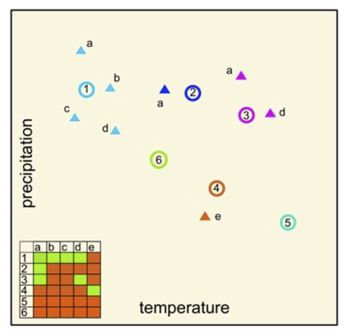
Figure 1. Schematic of a set of GCM/RCM simulations called “the matrix” (not based on real data) showing the response in temperature and precipitation in a system with 6 GCMs (circles, 1-6) and 5 RCMs (triangles, a-e). The matrix shows the available simulations in green, whereas missing simulations are in red. Note that this figure only shows the concept, and that there are many more GCM runs, but also downscaled experiments available (e.g. >70 in the EURO-CORDEX set). Also the “emptiness” of the matrix varies considerably per region and emission scenario.
RCMs are embedded in the output of GCMs, and typically can only be run for a (often rather small) sub-selection of the available GCMs (see Fig. 1 for a hypothetical example). This implies that not all possible large-scale future climate states (as simulated by the GCMs) are covered with the current set of RCMs. This could introduce a bias in the climate response in the RCMs with respect to the GCMs as well as “unexplored futures” that may be important from a certain user risk perspective. With international coordinated actions – like the EURO-CORDEX initiative – a large set of RCMs has been created in recent years, mitigating these problems to a considerable extent.
This is far more problematic for CPMs, which are computationally very demanding and therefore can only simulate rather short time slices of typically 10-30 years. Despite large efforts in Work Package 3 of EUCP to produce these simulations, they are still a so-called ensemble of opportunity, and no effort has been made to systematically explore the GCM uncertainty range. This limits the straightforward applicability of CPM results, and careful analysis has to be made to extract the useful information. For instance, though changes in convective rain statistics on a specific location are dominated by large uncertainty due to random climate noise, robust changes can be obtained by spatially pooling larger areas.
The other main aim of Task 5.4 is to investigate how to deal with the fact that we have only a relatively small set of downscaling experiments, given the wealth of GCM simulations available in CMIP5 and CMIP6. Methods are being developed that aim to statistically fill in, or emulate, these gaps in the matrix (red blocks in Fig. 1). This work is still very experimental: uncertainties in the appropriate large-scale predictors and how to combine them using statistical methods are still abundant. Methods range from very simple interpolation methods such as pattern scaling (DMI/NBI) to rather advanced methods using neural network machine learning techniques based on various large-scale predictors (CNRM).
Given the diversity of these approaches – in methodology, input, and what they can emulate – a simple common framework to test and compare them has been designed. In this framework a mid-century climate is emulated using information from the present-day and an end-century climate scenario (RCP8.5), using three models: CNRM-CM5 r1i1p1@150km (GCM), CNRM-ALADIN63@12km (RCM) and CNRM-AROME41t1@2.5km (CPM). One preliminary outcome appears to be that there is no one-size-fits-all solution, and more advanced methods do not necessarily provide more realistic outcomes for all evaluation measures. Yet, advanced methods such as machine learning clearly have a better range of applicability, for instance by providing daily time series with realistic variability (which cannot be done by most simple methods). Besides comparing different methods, another aim of the common framework is to develop simple statistical measures of the quality of emulated climate. This work is in progress and more outcomes are expected later in 2021.

 Funded by the European Union under Horizon 2020.